Get started with allometree
Song, Xiao Ping
2022-03-22
Source:vignettes/allometree.Rmd
allometree.RmdThe allometree package enables you to develop and use allometric equations relating to the size and structure of urban trees. For example, these equations have been used to predict trunk diameter from tree age, as well as to predict tree height, crown height, crown diameter and leaf area from trunk diameter. They are foundational to other models that estimate the benefits and hazards associated with trees as they mature and grow in size.
This document demonstrates the workflow to develop these allometric models, taking the relationship between two size parameters as an example: Predicting tree height from trunk diameter.
Two linear modelling approaches will be introduced:
- Regression models developed separately for each species, i.e., single-species models
- Mixed-effects model that includes all species as random effects, i.e., mixed-effects model
Example data: urbantrees
We will be using data(urbantrees). It contains five species planted along streets in Singapore, each spanning a wide range of heights and diameter sizes (in metres).
data(urbantrees, package = "allometree")
urbantrees
#> # A tibble: 1,584 × 3
#>    species                  diameter height
#>    <chr>                       <dbl>  <int>
#>  1 Hopea odorata              0.0987      4
#>  2 Hopea odorata              0.108       4
#>  3 Hopea odorata              0.111       4
#>  4 Xanthostemon chrysanthus   0.191       5
#>  5 Xanthostemon chrysanthus   0.150       5
#>  6 Xanthostemon chrysanthus   0.137       5
#>  7 Xanthostemon chrysanthus   0.207       5
#>  8 Xanthostemon chrysanthus   0.162       5
#>  9 Xanthostemon chrysanthus   0.134       5
#> 10 Xanthostemon chrysanthus   0.105       3
#> # … with 1,574 more rows

library(ggplot2)

ggplot(urbantrees, aes(diameter, height)) +
  facet_wrap(~ species, scales = "free") +
  geom_point(size=0.35, alpha = 0.3, color = "grey50") +
  theme_bw() + theme(panel.grid = element_blank())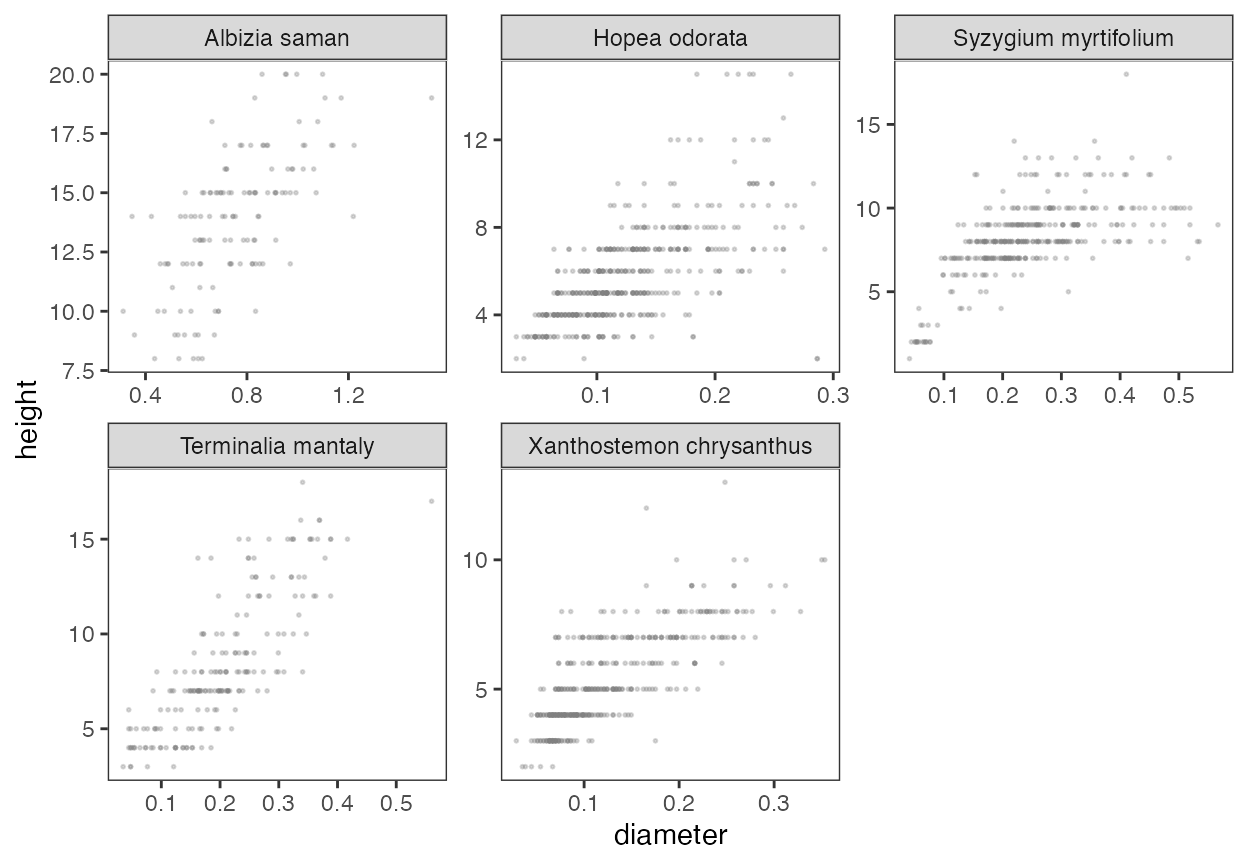
Allometric equations: eqns_info
Allometric relationships for urban trees can vary drastically from those for forest trees, and are also influenced by human factors such as pruning and fertilisation. Empirical models are developed using six allometric equations used for urban trees (McPherson et al., 2016).
More information can be found in ?eqns_info, as well as in data(eqns_info). The column modelcode shows the unique model code for each equation:
data(eqns_info, package = "allometree")
head(eqns_info)
#>   modeltype    base_equation   base_formula      weights modelcode
#> 1    Linear       y = a + bx          y ~ x                 lin_w1
#> 2    Linear       y = a + bx          y ~ x I(1/sqrt(x))    lin_w2
#> 3    Linear       y = a + bx          y ~ x       I(1/x)    lin_w3
#> 4    Linear       y = a + bx          y ~ x     I(1/x^2)    lin_w4
#> 5 Quadratic y = a + bx + x^2 y ~ x + I(x^2)                quad_w1
#> 6 Quadratic y = a + bx + x^2 y ~ x + I(x^2) I(1/sqrt(x))   quad_w2
1. Single-species models
We can run ss_modelselect_multi() to select the best-fit model for each species in the dataset urbantrees. This can also be done for individual species using ss_modelselect(). Note that you can also fit data to specified (i.e. pre-defined) equations, using the functions ss_modelfit() and ss_modelfit_multi(). This can be done, for example, after the removal of outliers from the full dataset. See the vignette Single-species linear models for a full demonstration.
results <- ss_modelselect_multi(urbantrees,
                                species = "species", # specify colname of species
                                response = "height", predictor = "diameter") # specify colnames of variables
results is a list of 3 elements:
- List of tables showing each species’ candidate models ranked by Aikake’s Information Criterion corrected for small sample sizes (AICc), named
ss_models_rank. - List of each species’ best-fit model object, named
ss_models. - Table showing each species’ best-fit model information, named
ss_models_info.
An overview of the best-fit models across the 5 species:
results$ss_models_info
#>                    species modelcode         a           b          c        d
#> 1            Albizia saman    lin_w1  6.717431   9.4640964         NA       NA
#> 2            Hopea odorata  quart_w4 -1.149669 149.3178483 -1522.6122 7908.410
#> 3     Syzygium myrtifolium  quart_w2 -4.614100 158.5128488  -748.2492 1638.676
#> 4       Terminalia mantaly   expo_w1  1.241983   3.8600410         NA       NA
#> 5 Xanthostemon chrysanthus loglog_w1  2.947907   0.5916555         NA       NA
#>            e response_geom_mean correctn_factor predictor_min predictor_max
#> 1         NA          13.566083        1.000000    0.31194369     1.5278875
#> 2 -14225.442           5.390829        1.000000    0.03183099     0.2928451
#> 3  -1321.221           7.735643        1.000000    0.04138029     0.5665916
#> 4         NA           7.596013        1.000533    0.03501409     0.5602254
#> 5         NA           5.041605        1.000883    0.02864789     0.3533240
#>   response_min response_max residual_SE mean_SE adj_R2   n
#> 1            8           20      2.2050  4.7889 0.4276 133
#> 2            2           15     11.9430  2.6339 0.5460 483
#> 3            1           18      2.1674  2.2536 0.6662 353
#> 4            3           18      0.2493  0.0615 0.6702 197
#> 5            2           13      0.2123  0.0449 0.6137 418
We can simulate data across a range of diameter sizes for each species, and use their respective models to make predictions of tree height. The simulated data can also be extrapolated beyond the range used to fit the model, using the argument extrapolate. In this example, we specify that predictions should be made between the range 0 to 1 metre:
predictions_ss <- ss_simulate(ref_table = results$ss_models_info,
                              models = results$ss_models,
                              extrapolate = c(0,1))
head(predictions_ss)
#> # A tibble: 6 × 6
#> # Groups:   species [1]
#>   species       predictor   fit   lwr   upr extrapolated
#>   <chr>             <dbl> <dbl> <dbl> <dbl> <chr>
#> 1 Albizia saman     0.312  9.67  5.21  14.1 No
#> 2 Albizia saman     0.324  9.79  5.33  14.2 No
#> 3 Albizia saman     0.337  9.90  5.45  14.4 No
#> 4 Albizia saman     0.349 10.0   5.57  14.5 No
#> 5 Albizia saman     0.361 10.1   5.69  14.6 No
#> 6 Albizia saman     0.373 10.3   5.81  14.7 No
predictions_ss is a dataframe of simulated data for the diameter size (predictor) for each species. Other columns include the predicted height (fit), the lower (lwr) and upper (upr) bounds of the prediction interval, as well as whether the height/diameter variables are extrapolated beyond the original data used to fit the model.
Model predictions can be visualised alongside the original data using ggplot2::ggplot():
ggplot() +
  facet_wrap(~ species)+

  # raw data
  geom_point(data = urbantrees,
             aes(x = diameter, y = height),
             size=0.35, alpha = 0.3, color = "grey50") +

  # prediction interval
  geom_ribbon(data = predictions_ss,
              aes(x = predictor, ymin = lwr, ymax = upr),
              alpha = 0.10) +

  # regression line
  geom_line(data = predictions_ss,
            aes(x = predictor, y = fit, lty = extrapolated)) +
  scale_linetype_manual(values=c("No"= 1 , "Low" = 3, "High" = 3),
                        name = "Extrapolated") +

  # axes
  xlab("Diameter (m)") + ylab("Height (m)") +
  coord_cartesian(ylim=c(0, max(urbantrees$height)), # limit ranges
                  xlim= c(0, max(predictions_ss$predictor))) +

  theme_bw() + theme(panel.grid = element_blank())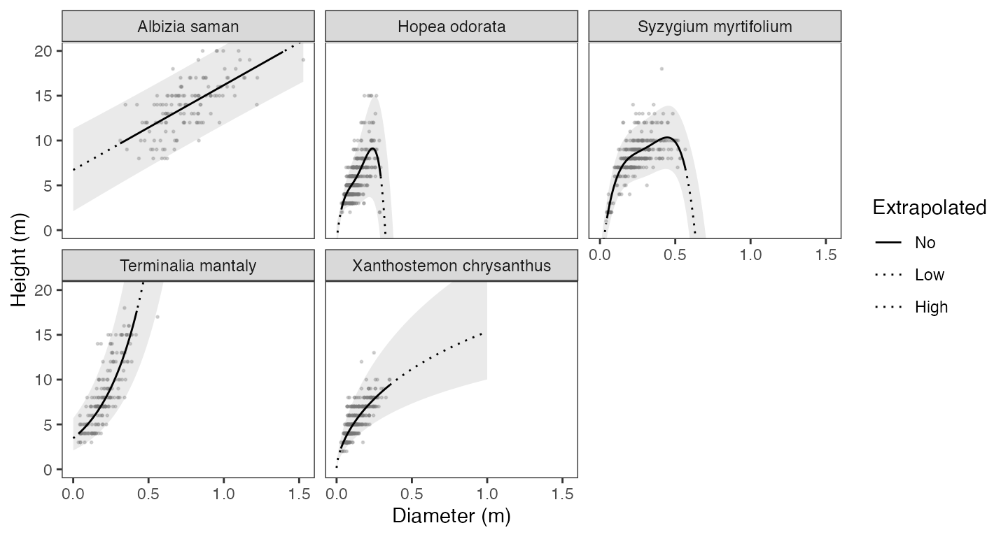
2. Mixed-effects model
Alternatively, the full dataset can be fit to a linear mixed-effects model with ‘species’ specified as the random effect, using the lme4::lmer function under the hood.
results <- mix_modelselect(urbantrees,
                           species = "species",
                           response = "height", predictor = "diameter")
results is a list of 5 elements:
- Model selection table showing all the types of mixed-effects models considered, ranked in order of ascending AICc.
- The best-fit model object, named
best_model. - The conditional and marginal pseudo- of the best-fit model.
- Correction factor used to adjust predicted values if response variable is transformed (incorporated into reported parameters).
- Warning messages, if any, spit from the models.
Simulations can likewise be performed across a range of diameter sizes for each species, and extrapolated beyond the range used to fit the model:
predictions_mix <- mix_simulate(data = urbantrees,
                                modelselect = results,
                                extrapolate = c(0, 1))
head(predictions_mix)
#>         species   predictor extrapolated       fit       upr       lwr
#> 1 Albizia saman 0.000000000          Low 0.0000000 0.0000000 0.0000000
#> 2 Albizia saman 0.003150946          Low 0.6474250 0.9599675 0.4169782
#> 3 Albizia saman 0.006301893          Low 0.9776586 1.4278679 0.6671479
#> 4 Albizia saman 0.009452839          Low 1.2505526 1.7209196 0.8677478
#> 5 Albizia saman 0.012603785          Low 1.4549722 2.0377412 1.0504206
#> 6 Albizia saman 0.015754732          Low 1.6879139 2.3592675 1.1863967
Model predictions can be visualised alongside the original data using ggplot2::ggplot():
ggplot() +
  facet_wrap(~ species)+

  # raw data
  geom_point(data = urbantrees,
             aes(x = diameter, y = height),
             size=0.35, alpha = 0.3, color = "grey50") +

  # prediction interval
  geom_ribbon(data = predictions_mix,
              aes(x = predictor, ymin = lwr, ymax = upr),
              alpha = 0.10) +

  # regression line
  geom_line(data = predictions_mix,
            aes(x = predictor, y = fit, lty = extrapolated)) +
  scale_linetype_manual(values=c("No"= 1 , "Low" = 3, "High" = 3),
                        name = "Extrapolated") +

  # axes
  xlab("Diameter (m)") + ylab("Height (m)") +
  coord_cartesian(ylim=c(0, max(urbantrees$height)), # limit ranges
                  xlim= c(0, max(predictions_mix$predictor))) +

  theme_bw() + theme(panel.grid = element_blank())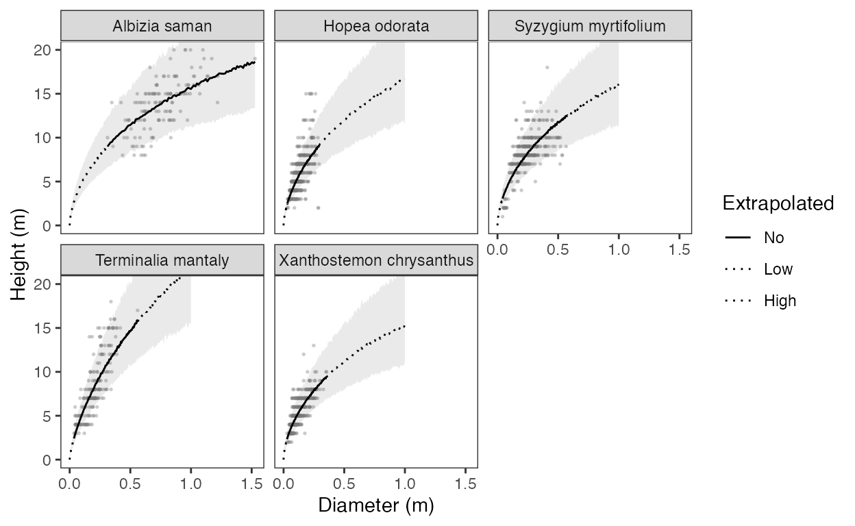
References
McPherson E. G., van Doorn N. S. & Peper P. J. (2016) Urban Tree Database and Allometric Equations. General Technical Report PSW-GTR-253, USDA Forest Service, 86.
Song, X. P., Lai, H. R., Wijedasa, L. S., Tan, P. Y., Edwards, P. J., & Richards, D. R. (2020), Height–diameter allometry for the management of city trees in the tropics. Environmental Research Letters, 15, 114017. https://doi.org/10.1088/1748-9326/abbbad